
After a very brief comment about needing to operationalise 'better', I decided that rather than reading book proofs I'd do a tongue in cheek analysis of what is better max or no max and here it is.
First we need to operationalise 'better'. I have done this by accepting subjective opinion as determining 'better' and specifically ratings of albums on amazon.com (although I am English metal sucks is US based, so I thought I'd pander to them and take ratings from the US site). Our questions then becomes 'is max or no max rated higher by the sorts of people who leave reviews on Amazon'. We have operationalised our questions and turned it into a scientific statement, which we can test with data. [There are all sorts of problems with using these ratings, not least of which is that they tend to be positively biased, and they likely reflect a certain type of person who reviews, often reviews reflect things other than the music (e.g., arrived quickly 5*), and so on ... but fuck it, this is not serious science, just a bit of a laugh.]
Post Sepultura: Max or No Max
The first question is whether post-max Sepultura or Soulfly are rated higher. Figure 1 shows that the data are hideously skewed with people tending to give positive reviews and 4-5* ratings. Figure 2 shows the mean ratings by year post Max's departure (note they released albums in different years so the dots are out of synch, but it's a useful timeline). Figure 2 seems to suggest that after the first couple of albums, both bands are rated fairly similarly: the Soulfly line is higher but error bars overlap a lot for all but the first albums.
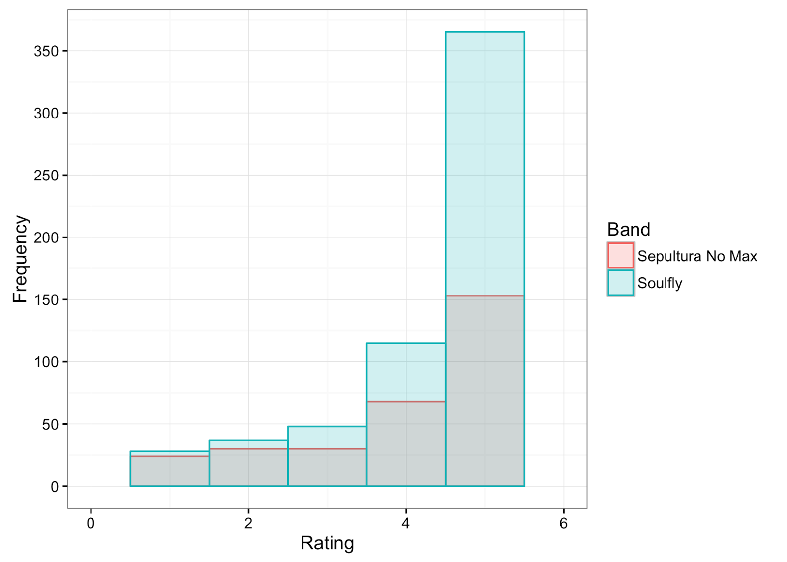 | ||
| Figure 1: Histograms of all ratings for Soulfly and (Non-Max Era) Sepultura |
 | ||
| Figure 2: Mean ratings of Soulfly and (Non-Max Era) Sepultura by year of album release |
I'm going to fit three models. The first is an intercept only model (a baseline with no predictors), the second allows intercepts to vary across albums (which allows ratings to vary by album, which seems like a sensible thing to do because albums will vary in quality) the third predicts ratings from the band (Sepultura vs Soulfly).
maxModel2a<-gls(Rating ~ 1, data = sepvssoul, method = "ML")
maxModel2b<-lme(Rating ~ 1, random = ~1|Album, data = sepvssoul, method = "ML")
maxModel2c<-update(maxModel2b, .~. + Band)
anova(maxModel2a, maxModel2b, maxModel2c)
By comparing models we can see:
Model df AIC BIC logLik Test L.Ratio p-value
maxModel2a 1 2 2889.412 2899.013 -1442.706
maxModel2b 2 3 2853.747 2868.148 -1423.873 1 vs 2 37.66536 <.0001
maxModel2c 3 4 2854.309 2873.510 -1423.155 2 vs 3 1.43806 0.2305
That album ratings varied very significantly (not surprising), the p-value is < .0001, but that band did not significantly predict ratings overall (p = .231). If you like you can look at the summary of the model by executing:
summary(maxModel2c)
Which gives us this output:
Linear mixed-effects model fit by maximum likelihood
Data: sepvssoul
AIC BIC logLik
2854.309 2873.51 -1423.154
Random effects:
Formula: ~1 | Album
(Intercept) Residual
StdDev: 0.2705842 1.166457
Fixed effects: Rating ~ Band
Value Std.Error DF t-value p-value
(Intercept) 4.078740 0.1311196 882 31.107015 0.0000
BandSoulfly 0.204237 0.1650047 14 1.237765 0.2362
Correlation:
(Intr)
BandSoulfly -0.795
Standardized Within-Group Residuals:
Min Q1 Med Q3 Max
-2.9717684 -0.3367275 0.4998698 0.6230082 1.2686186
Number of Observations: 898
Number of Groups: 16
The difference in ratings between Sepultura and Soulfly was b = 0.20. Ratings for soulfully were higher, but not significantly so (if we allow ratings to vary over albums, if you take that random effect out you'll get a very different picture because that variability will go into the fixed effect of 'band'.).
Max or No Max
Just because this isn't fun enough, we could also just look at whether either Sepultura (post 1996) or Soulfly can compete with the Max-era-Sepultura heyday.
I'm going to fit three models but this time including the early Sepultura albums (with max). The models are the same as before except that the fixed effect of band now has three levels: Sepultura Max, Sepultura no-Max and Soulfly:
maxModela<-gls(Rating ~ 1, data = maxvsnomax, method = "ML")
maxModelb<-lme(Rating ~ 1, random = ~1|Album, data = maxvsnomax, method = "ML")
maxModelc<-update(maxModelb, .~. + Band)
anova(maxModela, maxModelb, maxModelc)
By comparing models we can see:
Model df AIC BIC logLik Test L.Ratio p-value
maxModela 1 2 4686.930 4697.601 -2341.465
maxModelb 2 3 4583.966 4599.973 -2288.983 1 vs 2 104.96454 <.0001
maxModelc 3 5 4581.436 4608.114 -2285.718 2 vs 3 6.52947 0.0382
That album ratings varied very significantly (not surprising), the p-value is < .0001, and the band did significantly predict ratings overall (p = .038). If you like you can look at the summary of the model by executing:
summary(maxModelc)
Which gives us this output:
Linear mixed-effects model fit by maximum likelihood
Data: maxvsnomax
AIC BIC logLik
4581.436 4608.114 -2285.718
Random effects:
Formula: ~1 | Album
(Intercept) Residual
StdDev: 0.25458 1.062036
Fixed effects: Rating ~ Band
Value Std.Error DF t-value p-value
(Intercept) 4.545918 0.1136968 1512 39.98281 0.0000
BandSepultura No Max -0.465626 0.1669412 19 -2.78916 0.0117
BandSoulfly -0.262609 0.1471749 19 -1.78433 0.0903
Correlation:
(Intr) BndSNM
BandSepultura No Max -0.681
BandSoulfly -0.773 0.526
Standardized Within-Group Residuals:
Min Q1 Med Q3 Max
-3.3954974 -0.3147123 0.3708523 0.6268751 1.3987442
Number of Observations: 1534
Number of Groups: 22
The difference in ratings between Sepultura without Max compared to with him was b = -0.47 and significant at p = .012 (ratings for post-max Sepultura are significantly worse than for the Max-era Sepultura). The difference in ratings between Soulfly compared two Max-era Sepultura was b = -0.26 and not significant (p = .09) (ratings for Soulfly are not significantly worse than for the Max-era Sepultura). A couple of points here, p-values are silly, so don't read too much into them, but the parameter (the bs) which quantifies the effect is a bit smaller for Soulfly.
Confidence Intervals
Interestingly if you write yourself a little bootstrap routine to get some robust confidence intervals around the parameters:
data <- data[indices,] # select obs. in bootstrap sample
model <- lme(Rating ~ Band, random = ~1|Album, data = data, method = "ML")
fixef(model) # return coefficient vector
}
maxModel.boot<-boot(maxvsnomax, boot.lme, 1000)
maxModel.boot
boot.ci(maxModel.boot, index = 1, type = "perc")
boot.ci(maxModel.boot, index = 2, type = "perc")
boot.ci(maxModel.boot, index = 3, type = "perc")
Then you find these confidence intervals for the three betas (intercept, Post-Max Sepultura vs. Max Era-Sepultura, Soulfly vs. Max-Era-Sepultura):
BOOTSTRAP CONFIDENCE INTERVAL CALCULATIONS
Based on 1000 bootstrap replicates
CALL :
boot.ci(boot.out = maxModel.boot, type = "perc", index = 1)
Intervals :
Level Percentile
95% ( 4.468, 4.620 )
Calculations and Intervals on Original Scale
BOOTSTRAP CONFIDENCE INTERVAL CALCULATIONS
Based on 1000 bootstrap replicates
CALL :
boot.ci(boot.out = maxModel.boot, type = "perc", index = 2)
Intervals :
Level Percentile
95% (-0.6153, -0.3100 )
Calculations and Intervals on Original Scale
BOOTSTRAP CONFIDENCE INTERVAL CALCULATIONS
Based on 1000 bootstrap replicates
CALL :
boot.ci(boot.out = maxModel.boot, type = "perc", index = 3)
Intervals :
Level Percentile
95% (-0.3861, -0.1503 )
Calculations and Intervals on Original Scalens: 1534
Number of Groups: 22
The difference in ratings between Sepultura without Max compared to with him was b = -0.47 [-0.62, -0.31]. The difference in ratings between Soulfly compared to Max-era Sepultura was b = -0.26 [-0.39, -0.15]. This suggests that both soulfully and post-Max Sepultura yield negative parameters that reflect (to the degree that you believe that a confidence interval tells you about the population parameter ....) a negative effect in the population. In other words, both bands are rated worse than Max-era Sepultura.
Summary
Look, this is just a bit of fun and an excuse to show you how to use a bootstrap on a multilevel model, and how you can use data to try to answer pointless questions thrown at you on Twitter. Based on this hastily thrown together analysis that makes a lot of assumptions about a lot of things, my 120 character twitter response will be: Sepultura Max better than everything, but post 1996 Max is no better than No Max;-)
R Code
Data
You can generate the data using this R code (data correct as of today):
morbid<-c(rep(1,2), rep(2, 4), rep(3, 3), rep(4, 8), rep(5, 36))
Schizo<-c(rep(1,1), rep(2, 2), rep(3, 4), rep(4, 10), rep(5, 33))
remains<-c(2, rep(3, 5), rep(4, 9), rep(5, 104))
Arise<-c(rep(2, 2), rep(4, 16), rep(5, 89))
Chaos<-c(rep(1,4), rep(2, 2), rep(3, 9), rep(4, 20), rep(5, 120))
Roots<-c(rep(1,9), rep(2, 8), rep(3, 17), rep(4, 24), rep(5, 94))
Against<-c(rep(1,16), rep(2, 14), rep(3, 11), rep(4, 20), rep(5, 32))
Nation<-c(rep(1,3), rep(2, 7), rep(3, 6), rep(4, 22), rep(5, 19))
Roorback<-c(rep(1,6), rep(2, 6), rep(3, 5), rep(4, 13), rep(5, 20))
Dante<-c(rep(1,1), rep(2, 3), rep(3, 4), rep(4, 8), rep(5, 30))
Alex<-c(rep(1,1), rep(2, 1), rep(3, 3), rep(4, 6), rep(5, 18))
Kairos<-c(rep(1,3), rep(2, 2), rep(3, 2), rep(4, 6), rep(5, 33))
Mediator<- c(rep(1,0), rep(2, 3), rep(3, 4), rep(4, 6), rep(5, 21))
morbid<-data.frame(rep("Morbid", length(morbid)), rep(1986, length(morbid)), morbid)
Schizo<-data.frame(rep("Schizo", length(Schizo)), rep(1987, length(Schizo)), Schizo)
Remains<-data.frame(rep("remains", length(remains)), rep(1989, length(remains)), remains)
Arise<-data.frame(rep("Arise", length(Arise)), rep(1991, length(Arise)), Arise)
Chaos<-data.frame(rep("Chaos", length(Chaos)), rep(1993, length(Chaos)), Chaos)
Roots<-data.frame(rep("Roots", length(Roots)), rep(1996, length(Roots)), Roots)
Against<-data.frame(rep("Against", length(Against)), rep(1998, length(Against)), Against)
Nation<-data.frame(rep("Nation", length(Nation)), rep(2001, length(Nation)), Nation)
Roorback<-data.frame(rep("Roorback", length(Roorback)), rep(2003, length(Roorback)), Roorback)
Dante<-data.frame(rep("Dante", length(Dante)), rep(2006, length(Dante)), Dante)
Alex<-data.frame(rep("Alex", length(Alex)), rep(2009, length(Alex)), Alex)
Kairos<-data.frame(rep("Kairos", length(Kairos)), rep(2011, length(Kairos)), Kairos)
Mediator<-data.frame(rep("Mediator", length(Mediator)), rep(2013, length(Mediator)), Mediator)
names(morbid)<-c("Album", "Year", "Rating")
names(Schizo)<-c("Album", "Year", "Rating")
names(Remains)<-c("Album", "Year", "Rating")
names(Arise)<-c("Album", "Year", "Rating")
names(Chaos)<-c("Album", "Year", "Rating")
names(Roots)<-c("Album", "Year", "Rating")
names(Against)<-c("Album", "Year", "Rating")
names(Nation)<-c("Album", "Year", "Rating")
names(Dante)<-c("Album", "Year", "Rating")
names(Alex)<-c("Album", "Year", "Rating")
names(Kairos)<-c("Album", "Year", "Rating")
names(Mediator)<-c("Album", "Year", "Rating")
SepMax<-rbind(morbid, Schizo, Remains, Arise, Chaos, Roots)
SepMax$Band<-"Sepultura Max"
SepMax$Max<-"Max"
SepNoMax<-rbind(Against, Nation, Dante, Alex, Kairos, Mediator)
SepNoMax$Band<-"Sepultura No Max"
SepNoMax$Max<-"No Max"
soulfly<-c(rep(1,8), rep(2, 9), rep(3, 4), rep(4, 16), rep(5, 89))
primitive<-c(rep(1,11), rep(2, 5), rep(3, 5), rep(4, 19), rep(5, 53))
three<-c(rep(1,1), rep(2, 10), rep(3, 12), rep(4, 7), rep(5, 19))
prophecy<-c(rep(1,2), rep(2, 5), rep(3, 5), rep(4, 25), rep(5, 42))
darkages<-c(rep(1,1), rep(2, 1), rep(3, 5), rep(4, 18), rep(5, 36))
conquer<-c(rep(1,1), rep(2, 0), rep(3, 5), rep(4, 5), rep(5, 31))
omen<-c(rep(1,0), rep(2, 2), rep(3, 1), rep(4, 6), rep(5, 17))
enslaved<-c(rep(1,1), rep(2,1), rep(3, 4), rep(4, 2), rep(5, 30))
savages<-c(rep(1,0), rep(2, 2), rep(3, 3), rep(4, 10), rep(5, 27))
archangel<-c(rep(1,3), rep(2, 2), rep(3, 4), rep(4, 7), rep(5, 21))
soulfly<-data.frame(rep("Soulfly", length(soulfly)), rep(1998, length(soulfly)), soulfly)
primitive<-data.frame(rep("Primitive", length(primitive)), rep(2000, length(primitive)), primitive)
three<-data.frame(rep("Three", length(three)), rep(2002, length(three)), three)
prophecy<-data.frame(rep("Prophecy", length(prophecy)), rep(2004, length(prophecy)), prophecy)
darkages<-data.frame(rep("Darkages", length(darkages)), rep(2005, length(darkages)), darkages)
conquer<-data.frame(rep("Conquer", length(conquer)), rep(2008, length(conquer)), conquer)
omen<-data.frame(rep("Omen", length(omen)), rep(2010, length(omen)), omen)
enslaved<-data.frame(rep("Enslaved", length(enslaved)), rep(2012, length(enslaved)), enslaved)
savages<-data.frame(rep("Savages", length(savages)), rep(2013, length(savages)), savages)
archangel<-data.frame(rep("Archangel", length(archangel)), rep(2015, length(archangel)), archangel)
names(soulfly)<-c("Album", "Year", "Rating")
names(primitive)<-c("Album", "Year", "Rating")
names(three)<-c("Album", "Year", "Rating")
names(prophecy)<-c("Album", "Year", "Rating")
names(darkages)<-c("Album", "Year", "Rating")
names(conquer)<-c("Album", "Year", "Rating")
names(omen)<-c("Album", "Year", "Rating")
names(enslaved)<-c("Album", "Year", "Rating")
names(savages)<-c("Album", "Year", "Rating")
names(archangel)<-c("Album", "Year", "Rating")
Soulfly<-rbind(soulfly, primitive, three, prophecy, darkages, conquer, omen, enslaved, savages, archangel)
Soulfly$Band<-"Soulfly"
Soulfly$Max<-"Max"
maxvsnomax<-rbind(SepMax, SepNoMax, Soulfly)
maxvsnomax$Band<-factor(maxvsnomax$Band)
maxvsnomax$Max<-factor(maxvsnomax$Max)
maxvsnomax$Album<-factor(maxvsnomax$Album)
sepvssoul<-subset(maxvsnomax, Band != "Sepultura Max")
sepvssoul$Band<-factor(sepvssoul$Band)
sepvssoul$Album<-factor(sepvssoul$Album)
Graphs in this post
library(ggplot2)
m <- ggplot(sepvssoul, aes(x = Rating, fill = Band, colour = Band))
m + geom_histogram(binwidth = 1, alpha = .2, position="identity") + coord_cartesian(xlim = c(0, 6)) + scale_y_continuous(breaks = seq(0, 400, 50)) + labs(x = "Rating", y = "Frequency", colour = "Band", fill = "Band") + theme_bw()
line <- ggplot(sepvssoul, aes(Year, Rating, colour = Band))
line + stat_summary(fun.y = mean, geom = "point") + stat_summary(fun.data = mean_cl_boot, geom = "errorbar", width = 0.2) + labs(x = "Year", y = "Mean Rating on Amazon.com") + coord_cartesian(ylim = c(1, 5)) + scale_x_continuous(breaks=seq(1998, 2015, 1))+ theme_bw() + stat_summary(fun.y = mean, geom = "line", aes(group=Band))